Create an Amazing Stock Portfolio Spreadsheet (Excel)

---

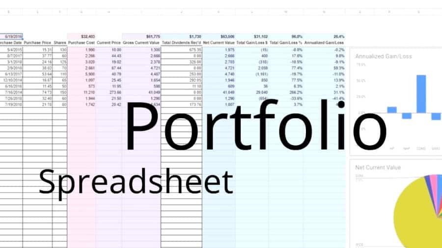
• Using Google Sheets or Excel, you can build a custom spreadsheet that will allow you to see the information about your investments that matters most
• There are many tools online for investors to monitor their portfolios
  • They might not have information formatted in the way you want or illustrated in the way you want
  • Spreadsheets allow you to make a portfolio analysis tool that is exactly the way you want it

Would you rather watch a video than read a tutorial? Check out these posts:
TRACK YOUR STOCK PORTFOLIO RETURNS USING GOOGLE SHEETS (OR EXCEL) – STEP BY STEP TUTORIAL

5 SUPPORT VIDEOS FOR THE EXCEL STOCK PORTFOLIO SPREADSHEET

Save some time and download a copy of the Portfolio Spreadsheet here!

Don’t feel like DIY-ing it?

Complete the form below and click Submit.
A link to the Google Sheet will be emailed to you.

Once you’re in the spreadsheet, click on File > Make a copy to edit. I’ll no longer be responding to “Requests for access.”

How to make a stock portfolio in Excel, Google Sheets, or any other spreadsheet software

This “how-to” can be followed along in either Excel or Google Sheets. Really, any spreadsheet software will do. The formulas should be the same. Also, formatting and charting options should be very similar.

I will be using Google Sheets in this tutorial. I like Excel and use it often. Particularly with some of my more “intensive” models. In this case, however, I think that Google Sheets is a better option. First and foremost because of its GOOGLEFINANCE functionality which will automatically update certain fields for you (price, volume, PE, EPS, and on, and on…). Second, since Google Sheets is cloud-based, you can access it anywhere – including your mobile device.

Microsoft does have a cloud-based version of Office (Excel), but I would not recommend it. I am a Microsoft fan in general and a big Excel fan in particular. But, I thought Office 365 (or whatever it’s called) fell way short. Just my opinion though, use whatever you’re most comfortable with.

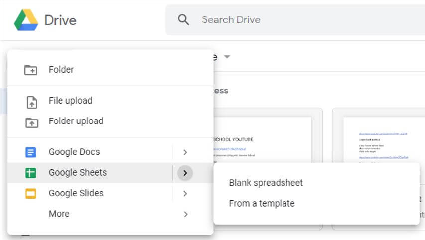
In order to follow along in Google Sheets, you’ll need a Google account. If you don’t already have one, click here for instructions on how to set one up.

Once you have your Google account set up, go to Google Drive and select “New” in the upper left-hand corner. Click on “Google Sheets > Blank spreadsheet”.

Okay, you should be ready to go, so let’s get into it.

Want to know how to add quality stocks to your portfolio? Read this post:
DETAILED STOCK VALUATION SPREADSHEET WITH WALK-THROUGH

First things first – enter your headers

Before you enter any information about your stocks or any formulas for calculations, you’ll want to lay the foundation of the spreadsheet by determining what information you want to see.

For this example, things were kept relatively simple. The amount of information you can glean from an investment’s current or historical data is almost limitless.

But, since this how-to is meant to serve as a starting point, I tried to keep things elementary. Here’s what we’ll analyze in this example:

• Company (fund) name
• Ticker symbol
• Purchase date
• Purchase price
• Shares
• Purchase cost
• Current price
• Gross current value
• Total dividends received
• Net current value
• Total gain or loss in dollars
• Total gain or loss percentage
• Annualized gain or loss

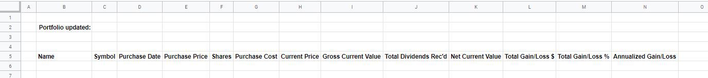
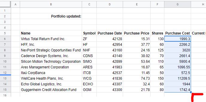
Enter these headers in the cells along the top of the spreadsheet. Personally, I like to leave a little space at the top and the left-hand side of my spreadsheets. So, I’ll start in B5 and enter across to N5.

Additionally, I like to know the as-of date for when I last updated a workbook such as this. Therefore, in B2, I’ll enter “Portfolio updated:” and I’ll bold everything I just entered (Ctrl+B). Here’s what that looks like:

Want to track your dividend stocks’ yield, income, and growth? Read this post:
CREATE AN AMAZING DIVIDEND TRACKING SPREADSHEET

Input some basic stock data

As mentioned earlier, this portfolio spreadsheet will consist of information you already know and information that you need to calculate.

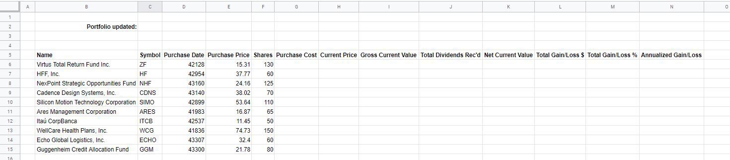
The Name, Symbol, Purchase Date, Purchase Price, and Shares fields are all information you should already have. So, go ahead and enter that.

All of this information, in my example, was chosen at random. You may have more stocks or fewer stocks.

Google Sheets and Excel can certainly handle everything you have in your portfolio.

It might take some digging on your part to unearth this information – even if you have an online broker. Particularly the Purchase Date. But, if you want an accurate calculation of your Annualized Gain/Loss do your best to find it.

What if I have different Purchase Dates for different lots of the same stock?

That’s a bit of a conundrum. To be completely honest, you might want a more sophisticated portfolio spreadsheet. But, there are a couple of ways you might work around it.

First, you could just list each lot separately. The only potential problem here is when it comes to allocating dividends (if any) to the different lots.

Second, you could group all of the lots together. But, unless you calculate a weighted-average Purchase Date and Purchase Price, a lot of your calculations are going to be erroneous.

Personally, I would separate the lots out and then group all of the dividend information under the lot you purchased first – for simplicity’s sake.

Here’s what we have so far:

Formula time! Purchase Cost

We’ll start off simple.

Purchase Cost = Purchase Price × Shares

At the risk of oversimplifying things – I’ll clarify for those of you who are completely new to spreadsheets…

Every formula begins with an equal sign (=). That’s how Google Sheets and Excel know to perform a calculation.

So, in cell G6, type “=E6*F6” and press Enter. The asterisk (*) means multiply.

In my example, for stock symbol ZF, the result is $1,990 ($15.31 Purchase Price times 130 Shares).

Don’t type more than you need to, copy down!

Now, you need to duplicate this formula for every stock in your portfolio.

But, don’t go to row 7 and type “=E7*F7”. Then row 8 and type “=E8*F8”. And so on…

Either copy the formula in G6 (Ctrl + C) and then paste (Ctrl + V) in cells G7 through G50 (or whatever row you end on).

Or, alternatively, Google Sheets and Excel give you the ability to duplicate what’s in a cell (the formula) by clicking on the little square in the lower right-hand of the active cell, holding the mouse button down, and dragging it where you want it to copy. This is the quickest and easiest way to do it.

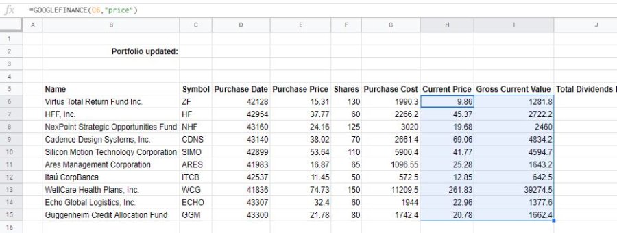
Automate Current Price and Gross Current Value in Google Sheets

One of the reasons I elected to use Google Sheets for this tutorial is because of the GOOGLEFINANCE function. I know that Excel used to have MSN Money functionality. But, if they currently have something similar, I’m not familiar with it.

What is GOOGLEFINANCE?

It gives you the ability to connect to Google Finance through a formula and populate Google Sheets with information about an individual stock.

For instance, if, in cell H6, you type “=GOOGLEFINANCE(C6,”price”)” the Current Price of the stock entered on row 6 will be populated and automatically updated. Note the equal sign (=), and the quotes around “price”. Don’t type the very first and very last quotes, though. Only type what’s in bold.

With the GOOGLEFINANCE function, you don’t have to worry about looking up the price (and other basic information, if you wish) and then manually typing it into Google Sheets! Always accurate and always up-to-date (though not real-time).

Copy the GOOGLEFINANCE function down for all of your stocks. If you’re using Excel, or otherwise opt not to utilize the GOOGLEFINANCE function, you’ll have to enter the Current Price manually.

With the Current Price, you can now calculate a Gross Current Value. Why “Gross?” Because, later, we’ll add dividends in order to get a Net Current Value.

Gross Current Value = Shares × Current Price

In cell I6, type the following formula: “=F6*H6”. Copy that formula down for all of your stocks.

Here’s what it should look like thus far:

Dividends are an important part of your returns – be sure to include them!

Unfortunately, there’s no way (that I’m aware of ) to automatically import dividend data for the stocks you hold. Updating this information is by far the most labor-intensive step in this tutorial.

Yes, the GOOGLEFINANCE function can import the yield percentage for a given stock. But, since this stock portfolio spreadsheet is focused on total returns, that isn’t going to help much.

If you own your shares through an online brokerage, as most people do, you should be able to access dividend payment history for the individual stocks you own.

For example, TD Ameritrade allows you to display dividends paid for a specific stock in your transaction history.

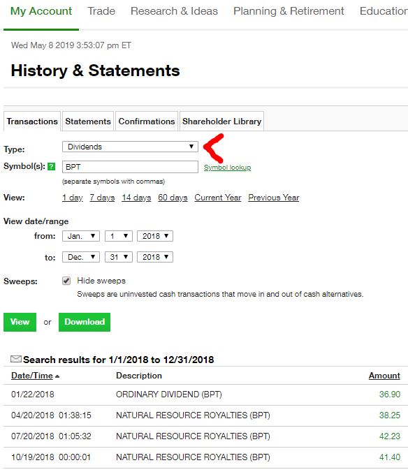
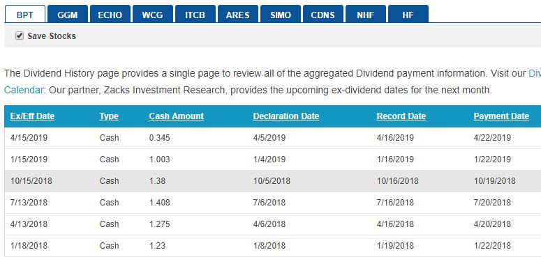
If this information can’t be easily retrieved from your brokerage, then you’ll have to do some homework. A good place to start would be the Nasdaq Dividend History page. Here, you can find the Payment Date and per share amounts of dividends paid for every stock. You’ll have to multiply the per share amounts by the number of shares owned to get the full dividend paid.

Total your dividends received for each of your stocks and enter that information under the Total Dividends Rec’d heading (column J).

For the sake of accuracy, make sure you only include dividends paid to you while you owned the stock. Also, be sure to update this information every time a stock pays a dividend.

It’s more trouble than it should be, for sure. But, as I said, dividends can make a huge contribution to the returns received for a particular stock. If this seems like too much trouble, you can forgo including dividends. Just know that your return numbers won’t be 100% accurate.

More about adding dividends to your stock tracker spreadsheet.

Totaling all of your returns

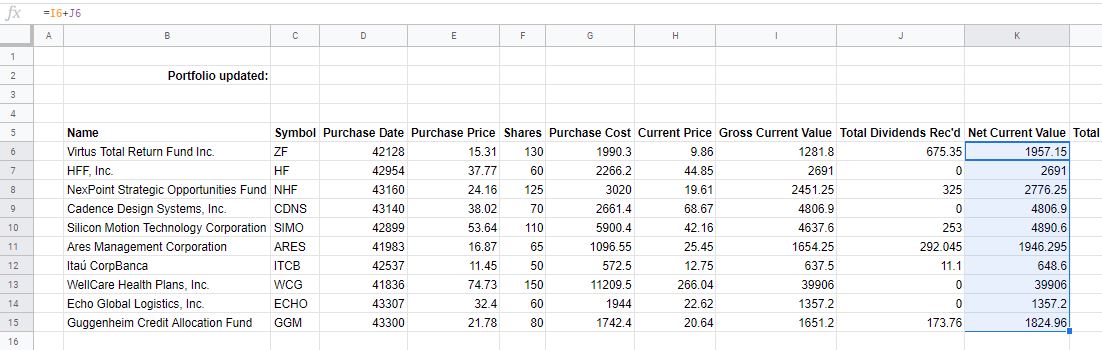
With dividend information gathered, you can now calculate the Net Current Value. This will total your returns from capital gains and from dividends and give you an accurate picture of the stock’s performance.

Net Current Value = Gross Current Value + Total Dividends Rec’d

In cell K6, enter the following: “=I6+J6”. Then, copy that formula down for the rest of your stocks.

Only a few more columns to go! Here’s what your stock portfolio should look like now:

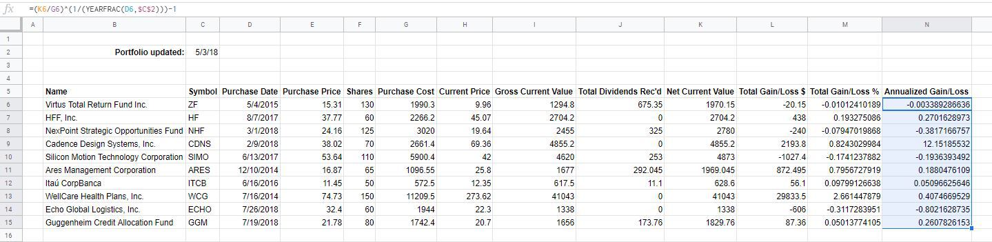
How are your stocks really doing?

The last three columns will be used to calculate the returns of each stock. Let’s focus on the first two columns first.

Total Gain/Loss $ = Net Current Value – Purchase Cost

This is the difference between the value of the stock now (including dividends received) and what you paid for it.

In cell L6, enter the following formula: “=K6-G6”. As usual, copy that down for the rest of the stocks.

Total Gain/Loss % = Total Gain/Loss $ ÷ Purchase Cost

In cell M6, type the following formula: “=L6/G6”. Copy it down…

This formula compares your Gain/Loss in dollars to what you paid for the shares of stock you own. The result is a percentage and it tells you what the total performance of your stock has been – thus far.

But, what’s a good Total Gain/Loss %? That’s difficult to answer. A 5% gain is good over the course of one day or one week. A 50% gain isn’t so good if it’s over the course of twenty years.

How to compare gains and losses – apples to apples

That’s why I think you should calculate the Annualized Gain/Loss.

I’ll warn ya, the formula is a little complicated. But, when you pull it off, it’ll provide valuable insight into the true performance of each stock. It will allow you to better compare stocks against one another.

Type the following in cell N6: “=(K6/G6)^(1/(YEARFRAC(D6,$C$2)))-1”.

Yikes!

You don’t have to necessarily know why it works. Just know that it does. Don’t let it scare you off, this will make more sense if I break it down.

Before we do that, make sure you have a Portfolio updated date in cell C2. This date is used to determine the amount of time that has passed since the stock was purchased and is critical for calculating Annualized Gain/Loss.

The first part of the formula, “(K6/G6)”, compares the Net Current Value to the Purchase Cost. It calculates the relationship between the value now and when you bought the stock.

The next part, “(1/(YEARFRAC(D6,$C$2)))” looks complicated, but, for the most part, all it’s doing is figuring the amount of time that has passed since you purchased the stock. What’s critical, though, is that you include the dollar signs ($) in front of the “C” and the “2”. This ensures that the formula is always comparing a stock’s Purchase Date to the same Portfolio updated date. The dollar signs ($) lock that cell into the formula so it doesn’t change when you copy it down.

Finally, the “-1” at the end turns the result of the equation into a percentage that makes sense.

That’s it! Again, the formula for cell N6 is: “=(K6/G6)^(1/(YEARFRAC(D6,$C$2)))-1”. Type that in. Copy it down. And, that nasty bit of business is over!

Here’s what it should look like with all of the information completed for each stock:

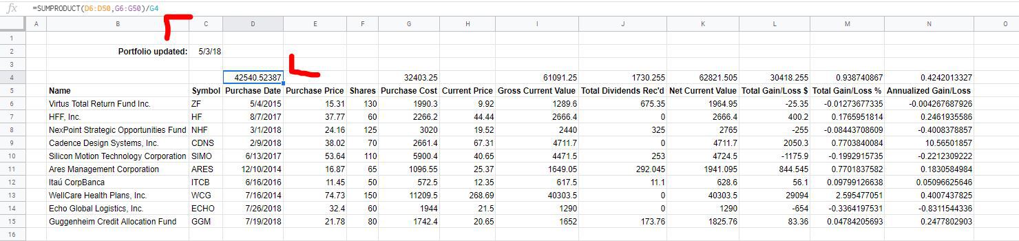
We’ve analyzed each stock – what about the overall portfolio?

While you could quit here and (with a little formatting) have a perfectly good stock portfolio spreadsheet – let’s push on just a bit further and put the final touches on this thing.

For most of our fields (except Current Price), we can analyze the portfolio in aggregate. That way you can compare your individual stocks against each other and understand how they contribute to the overall portfolio’s returns.

For most fields, this is pretty easy. It’s simply a matter of totaling the entire column. Others will use the exact same formula you used for individual stocks. One last field is a bit tricky to calculate for the entire portfolio – Purchase Date. But, let’s not get ahead of ourselves, let’s start with the easy ones…

Fields that are summarized with SUM

Purchase Cost, Gross Current Value, Total Dividends Rec’d, and Net Current Value amounts for the whole portfolio are simply sums of the amounts for each stock.

In order to sum these amounts, we’ll use the SUM function in Google Sheets/Excel. Start in cell G4 (above Purchase Cost) and enter the following: “=SUM(G6:G50)”.

You don’t have to stop on cell G50. If your list of stocks goes beyond row 50, then you can go to G100, G500, G1000, or however far down you need to. Just make sure that you are including the Purchase Cost for every stock in the equation. It will not hurt to include blank cells in the formula.

Enter the SUM function for Gross Current Value, Total Dividends Rec’d, and Net Current Value in row 4. E.g. “=SUM(I6:I50)”, “=SUM(J6:J50)”, and “=SUM(K6:K50)”.

Fields that are summarized with an equation

The Total Gain/Loss $, Total Gain/Loss %, and Annualized Gain/Loss fields use the same equations to calculate for the whole portfolio as they did for the individual stocks within.

Remember how you copied those formulas down rather than re-entering them for each stock? The same thing can be done with the portfolio calculations to save time.

Click and drag (highlight) across cells L6, M6, and N6, then press Ctrl+C (copy) on your keyboard. Then click on cell L4 and press Ctrl+V (paste). Viola! The spreadsheet will automatically use the previously calculated totals to determine Gain/Loss amounts for the entire stock portfolio.

One last formula…

Maybe you’re wondering how an Annualized Gain/Loss can be calculated for the entire portfolio if there’s no Purchase Date for the portfolio as a whole?

How the hell would you go about settling on one Purchase Date for a bunch of different stocks?

In order to pull this off, and get an accurate Annualized Gain/Loss for the entire stock portfolio, we need to calculate a weighted-average Purchase Date for the entire stock portfolio.

What will the Purchase Dates be weighted by? By Purchase Cost.

This is done by using a function in Google Sheets/Excel called SUMPRODUCT. No need to get into the particulars about how/why this works. Just know that it does. The result is a single Purchase Date for your entire portfolio.

In cell D4, enter the following formula: “=SUMPRODUCT(D6:D50,G6:G50)/G4”. Remember – if your list of stocks goes beyond row 50, change D50 and G50 to D100/G100, D150/G150…whatever you need to.

Don’t be alarmed if the result of that formula is a big number and not a date. That’s simply an issue of formatting and we’ll get into that next.

Here is what your (almost completed) stock portfolio spreadsheet should look like now:

This seems like good information, but it looks like crap!

Yep, you are correct. Time to spruce things up a little bit and make this information more readable.

Formatting is all a matter of preference. There’s no single right way to do it.

I’ll walk you through some of the things I like to do in terms of formatting and you can copy what you like. Also, feel free to explore on your own. Most of the formatting options are available below the main menu at the top of the spreadsheet. Mouse over the little icons, and you’ll see text pop up explaining what each option does.

I’d definitely say you want to format your Purchase Dates as dates – if they’re not already. Select those cells and click on the icon that has “123▼” on it. Lower down on the list, you should see a couple of options for a date format.

Another thing I almost always do when formatting a spreadsheet is to color in the cells that have formulas. That serves as a visual reminder, for me, not to type in them. The cells that are left white are the variables that can be changed. The little paint can icon is what you use to change cell color.

You can format the numerical data as numbers or currency. Show more or fewer decimals with the icons that have “.0←” or “.00→” on them.

I’d also change the Total Gain/Loss % and Annualized Gain/Loss to a percentage format. Use the “%” button on the menu.

Lastly, I like to bold my headers, and, usually, my totals.

Again, formatting is a matter of preference, so there are no wrong answers. Play around with it and make it look how you want. If you ever want to wipe the slate clean – select the cells you want to change, click on “Format” in the main menu, and then “Clear formatting.”

Below is how I opted to format my stock portfolio spreadsheet. You’ll notice the charts on the right-hand side. Which, we’ll get into next…

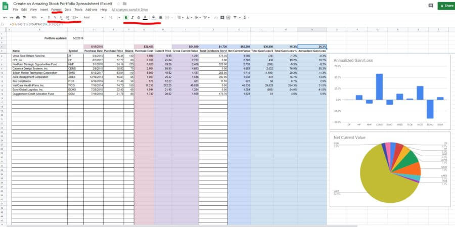
Use charts to better understand your portfolio and returns

You can chart anything on your spreadsheet. You could even create a bar chart comparing Purchase Prices or Shares if you wanted. Though, I’m not sure why you would?

In my spreadsheet, as you can see above, I opted to chart two things.

1. A comparison of the Annualized Gain/Loss among all of my stocks using a simple column chart
2. A pie chart that shows the composition of my portfolio – by stock

Creating these charts was quick and easy in Google Sheets. Doing so in Excel is also easy (“Insert”, then “Charts”). But, there will be some differences between the two visually.

To make the first chart, simply highlight all of your stock Symbols (not the header, C5). Then, holding down the Ctrl button, select all of the Annualized Gain/Loss percentages (again, not the header, N5). The Ctrl button allows you to select multiple cells that are not next to each other.

From the “Insert” menu, select “Chart.” You should see a column chart pop up with the Symbols in the x-axis and the percentages in the y-axis.

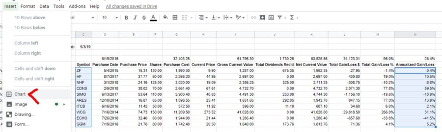
Click and drag the chart where you want it. If you double click it, you’ll see the Chart editor. After selecting “Customize” and then “Chart & axis titles” you can enter a title in the “Title text field.” As you can see, I just named mine Annualized Gain/Loss.

If you select the Symbols and Net Current Values and insert a chart, you’ll probably get another column chart. I think a pie graph better represents this information. Fortunately, changing the chart type is easy. Double click this new chart and in the Chart editor click “Setup” and change the “Chart type” by selecting a pie chart from the drop-down menu. It might be under the “SUGGESTED” heading.

There we go. A portfolio spreadsheet with well-formatted, useful information.

How to make a stock portfolio in Excel (or Sheets)

Spreadsheets allow users to analyze their portfolios and returns in just about any way imaginable. The GOOGLEFINANCE function in Sheets automates updates for a lot of frequently referenced information about stocks and mutual funds.

I tried to explain how my example stock portfolio was made in detail. What (if anything) did you get hung up on, though?

Is there additional information you would want to have in your stock portfolio spreadsheet? What would you want to analyze on an ongoing basis?

Join the conversation on Twitter!