Have a lot of dividend-paying stocks in your portfolio? Read this post:
CREATE AN AMAZING DIVIDEND TRACKING SPREADSHEET (EXCEL)
Video transcript – Stock portfolio
How to make a stock portfolio and Excel, Google Sheets, or any other spreadsheet software.
This how-to can be followed along in either Google Sheets or in Excel. Really any spreadsheet software will do fine. The formulas will be the same. The formatting and charting options should be very similar.
I’ll be using Google Sheets myself. I like Excel, and I use it often. But particularly with some of my more intensive models, I like Excel. But, in this case, however, I think that Google Sheets is a better option.
Firstly, because of its GOOGLEFINANCE functionality – which is a formula that automatically updates certain fields. You know, things like price, volume, P/E ratio, earnings per share, etc. A lot of others too.
And Google sheets is cloud-based which allows me to access this portfolio spreadsheet from anywhere. Microsoft does have a cloud-based version of Office and Excel. But I don’t really recommend it.
I’m a Microsoft fan in general and an Excel fan in particular, but that Office 365, or whatever, it is that they call it, fell way short. I just didn’t like it, but, by all means, use whatever you’re most comfortable with.
So, if you’re gonna follow along in Google Sheets you’ll need a Google account. if you don’t have one already then there’s the link in the post that you can follow that will take you to Google and walk you through how to set up a Google account.
Once you have that account set up then you’re gonna go to Google Drive and you’ll select New > Google Sheets. There’s a picture of that here and once you do that you’ll have a blank spreadsheet ready to go.
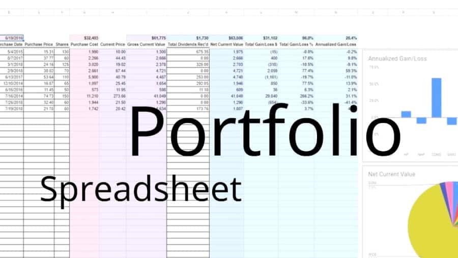
So, here’s the finished product. But, let’s walk through the steps to see how we got there.
First things first, you’re gonna enter your headers. This will lay the foundation so we know what information we’re either gonna have to go get or create formulas for.
In this example, I kept things pretty simple. You know, the amount of information that you could compile from an investment’s current or historical data is pretty much limitless. So, I wanted to keep things, in this instance, fairly simplistic.
Obviously, if you wanted to, you could always build upon this. This how-to is meant to be a starting point.
The pieces of information that I’m gonna compile are the company (or in some cases, it might be a mutual fund) name, the ticker symbol, the purchase price, shares, purchase cost, current price, gross current value (without dividends), total dividends received, net current value (which would include dividends), total gains and losses (in terms of dollars and in terms of percentage), and annualized gain and loss.
So, here you’re gonna enter these headers along row 5 and it will stretch from column B to column N.
I like to leave a little space at the top. But also, I want the room to put this in, and this is a place right here where you would enter when the portfolio was updated.
Okay, some of the cells I also bolded, as you can see. We do that too. But with all the headers entered then we can move on to some basic stock information.
This is all going to be information that you will know, or have access to. Simple to get your hands on.
If you don’t have access to it really easily, do what I did in my examples here – I chose stocks at random.
You may have more or fewer that’s fine. You’re not gonna have so many that you’ll run out of space on your spreadsheet.
If you have an online broker, you might need to use it to uncover some of this information. You know, particularly, the purchase date. But if you want an accurate calculation of the annualized gain in loss then that is information that you’re going to want to have.
So, here is where I typed all that information in.
In some cases, you might have different lots of stock. For instance, let’s look at my first stock I’ve listed here. It’s actually a closed-end fund, I think. That symbol is ZF.
Let’s say rather than purchasing all 130 shares on May 4th of 2015, I purchased a hundred shares on May 4th, 2014, and 30 shares on May 4th of 2015. I have a total of 130. But I purchased those in two separate transactions.
If this is something you’re gonna run into a lot, you might want a little more sophisticated portfolio spreadsheet than this one. As I said, this is kind of elementary, simplistic, you know…
But here are some ways you might work around it.
You can either list the lots separately. We can enter a lot of a hundred here and then, on a separate line, your lot of 30. The problem with that might be if you’re allocating dividends that you’ve received (which we’ll get to a little later). You might have an issue there.
Or, you can just group all the lots together. But, if you do that, and you don’t calculate a weighted average purchase date (which sounds weird because you don’t typically think of weighted averages when it comes to dates, but we’ll also touch on that a little bit more later) your gain and loss information is gonna be wrong.
The annualized gain and loss is particular. Personally, I would separate the lots out. And, then, just lump all the dividend information in with one of the lots. That’s probably the simplest way to go about it. But you can do whatever works best for you.
So, okay, we’ve got our basic information here: name, symbol, purchase date, purchase price, and the number of shares. Now we’ll get into some formulas.
We’ll start off simple. Here, we’re calculating purchase cost, and purchase cost is simply equal to purchase price times the number of shares, of course.
For those of you that are brand new to spreadsheets, I’ll kind of explain some of this. It’ll be simplistic. Maybe too simplistic for people who do have experience with spreadsheets. But, you know, like I said, this is a kind of a beginner’s tutorial so I’m trying to not scare anyone off here. If you aren’t new and are familiar with spreadsheets, then you know you can just hit the L button to jump ahead a couple of seconds. If some of the stuff is a little too elementary for you.
So, if you look up here and see the formula bar, every formula is gonna begin with an equal sign. You’re just gonna enter equals; and we’re doing purchase price, in this case for ZF, which would be E6 times F6. The asterisk is times, of course. If you enter that here, you’ll get your result. You see the formula still there in the formula bar. But this is what 15.31 times 130 is equal to $1,990.30.
You know, in this case, that wouldn’t include commission, of course. We’re just looking for the purchase cost for the stock itself.
But that’s all there is to it. So, equal C6 times F6.
Some you know that rather than typing that down in every single cell below the header, for every other stock, you can simply copy the formula down. So, you can either do Ctrl+C and highlight all those cells, then Ctrl+V. Or, you can use the little square in the lower right-hand corner here and drag it down like that and you can see that the spreadsheet, whether it’s Sheets or Excel, is smart enough to know what you want to do.
In this case, you know, you want to do the same thing for each line. Right here, see we’re taking E13 times F13, and it’s given us our purchase cost for WCG.
Now, we’ll get a little more into the GOOGLEFINANCE function that I mentioned earlier. This’ll automate the current price, and therefore the gross current value in Google sheets. As I said, that’s one of the reasons (the GOOGLEFINANCE function) that I opted to use Google Sheets.
I know that Excel used to have an MSN Money functionality, where you could do something similar. But I don’t know if they still have that.
The GOOGLEFINANCE function, you see it up here in the formula bar. And, what it basically does is it goes to Google Finance and connects to it with this formula. Then it populates Google Sheets with whatever information you tell it that you want.
So, for instance, here in H6 we typed =GOOGLEFINANCE then open parentheses. We specified our ticker. In this case, it says C6, which isn’t a real ticker. But, see our symbol is in C6, so we’re telling it to refer to C6 to go get that symbol.
Then the next thing we specified is that we wanted price. That’s the attribute that we want okay. You can see there’s a bunch of other stuff you can enter here. But don’t worry about that right now, just enter in H6 =GOOGLEFINANCE, open parentheses, refer to the cell (in this case is C6) as your symbol, and then enter “price” with parentheses around it, okay.
What’s nice about this is with this GOOGLEFINANCE function you don’t have to worry about looking at price and other basic information. Like I said earlier, manually typing into Google Sheets, you don’t have to go to Yahoo! Finance or Google Finance or wherever it might be that you get your price information. Then come in every day and type in a current price.
Okay, GOOGLEFINANCE will just go get it for you and updated it automatically.
Hit Enter here to make it visible here and then copy it down. Give it a second. There, you see it knows the current price for every single one of these symbols and we can calculate the gross current value.
Again, why are we calling it the gross current value? That’s because it’s not including any dividend information. So, the gross current value is simply F6 × H6. What that means is what’s in cell F6, or the number of shares. H6 is the current price that we got from the GOOGLEFINANCE function.
We enter that and there we go. 130 shares × 10.07, the current price. We got a gross current value of $1,309.10.
Rather than retyping the formula, we will just copy it down. And, there we go, the gross current value for every one of the stocks in your portfolio.
Dividends are obviously an important part of the return to that you receive it from a stock. So, we went to include that if we went to get accurate information about what our gains and losses have been for a particular stock.
Unfortunately, right now and there’s no way that I know of to automatically import dividend data for these stocks. Like through a GOOGLEFINANCE function, for instance. That would definitely be nice. A way might exist, I’m just not aware of it.
You know the GOOGLEFINANCE function can import the yield percentage for any given stock. But, that’s not really what we’re looking for. The yield is going to be over the past year, you know. But, you might have held the stock for more than one year.
Okay, so simply using the yield attribute with the GOOGLEFINANCE function isn’t going to do anything for us, unfortunately. This is just something that’s going to have to be entered manually. As you can see I already did that here are the time periods that I held these particular hypothetical stocks.
And, like I said you’ll notice up here in the formula bar it’s just an amount entered. There’s no formula, no equals, anything. It’s just the sum.
If we go over here to the post – if you own your shares through an online brokerage, then you probably have the ability to access dividend payment history for the stock. I use TD Ameritrade and show the screenshot here. I would imagine if you use a different broker, they offer something similar. Where you put in your date range specifically, you want to look at a dividend for your symbol, and it’ll give it all to you.
It’s really just a matter of going into your brokerage account and retrieving that information. Then, total the amounts of what you’re looking for.
You want the total amount of dividends that you’ve received since you’ve owned this particular stock.
If for whatever reason, you can’t get this information easily from your brokerage, then you’re going to have to do a little homework.
My suggestion would be to use the NASDAQ dividend history page. It will tell you the amount of the dividend paid for each share of a particular stock. Then, you want to multiply that by the number of shares you have to get the full amount you have received.
As I said, is annoying that it can’t be more of an automated sort of thing. But, that’s what we’re working with.
You can see here, you know, with the NASDAQ site it will show history for years and years in the past. Maybe, even, every dividend it’s ever paid.
Once you total those amounts, like I said, and threw them into the total dividends received column for each respective stock.
You know, make sure, for the sake of accuracy, that you’re only including dividends that we’re actually paid to you. Not dividends from before you owned the stock.
Be mindful of when you purchased it and, like I said, how much you receive.
It’s a lot of trouble, but dividends are an important part of your returns. So, we definitely want to include them.
Now, we’ll move on to the net current value, which will include all of what you’ve made through capital gains and losses. And include the dividends that you’ve received.
The formula here is just gross current value + total dividends received. So, you can see the formula bar here, we’ve got I6 +J6. And, that’ll give us the amount. In this case, $1,984.45.
Copy that down for the rest of the stocks. And there we got that current value now.
We want to know what the stocks are worth. We want to know how that relates to what we paid for it. So, we’re obviously going to compare what it’s worth now and the value we received versus what we paid for it.
This is the total gain and loss in dollars. Which is going to be that current value minus purchase cost. So, in cell I6 you’ll enter K6 – G6. That’s current value minus what you paid for it.
Okay, you know in this case $1,990.30. But, you know we bought at $15.31 for this particular stock. It’s gone down about 50% in value the $10.07.
But, we’ve received a decent amount of dividends since then. $675. So, that’s offset some of the loss in share value.
Total gains and losses then are $5.85. More or less broke even thanks to dividends, in this case.
So, enter that formula in I6, as I said. Copy it down for the rest of the stocks and measure your total gain and loss in dollars for each stock in your portfolio.
See here that I just chose the stocks at random for the purpose of an example. Collectively they’ve done pretty well.
The purchase price was $74.73, current price $285.69. So, in this case, I wish this wasn’t hypothetical. I wish I’d really bought this stock at $74.73. But, I did not.
Okay, we know the dollar amount of gain and loss now. We want to translate that into a percentage. You know, to be able to compare stocks between each other.
So, getting the total gain and loss in percentage is not too terribly hard. It’s just a matter of taking total gain and loss and dividing it by the purchase cost.
In this case, Cell M equals L6 ÷ G6. Total gain and loss in dollars ÷ purchase cost.
There, it’ll translate into a percentage now. If you’re formatting is a little different (getting numbers with lots of decimal points or in this case it’s not showing up as a percentage) it’s like .00312345, you know. Something like a big old weird-looking number. Don’t worry, we’ll talk about formatting here in a moment.
Like I said this formula compares your gain and loss in dollars to how much you paid for shares of the stock. It gives you the percentage gain and loss. That’s good information to have but it’s not complete.
What’s a good total gain and loss? It’s up to you. I know there’s no one answer for that.
A 5% gain is great if you’ve only held the stock for one day. Or even one week. On the other hand, a 50% gain isn’t so good if you’ve held the stock for 20 years.
So, like I said this information is incomplete and that’s why we have to include the last column. Annualized gain and loss (or CAGR).
This formula is a little more intensive and there’s really no way around it. What we’re doing here is translating this amount into what your gain and loss has been year-over-year.
The formulas up here it’s also on the post. Just copy and paste it if you want from the post. There’s no shame in doing that.
Or, you can type it out. But I won’t get into why this formula is what it is. It’s a little more in-depth and than I want to get into. It’s just to kind of give you an idea.
The first part compares what you paid versus the net current value. The net current value compares to the purchase cost. Really, the rest just determines the amount of time that’s passed since you purchased that stock.
If we go back look at the purchase dates, see that some we’ve held for 5 years and some for less than one year. If you go ahead and keep your portfolio updated you’ll need it for this particular formula.
Make sure you’ve got today’s date in here and this isn’t today’s date so I actually I’ll leave that it May 3rd. That’s when I created the post. I’ll show you how to change it when I update that date.
Again, this formula on. Don’t let it scare you off. Copy and paste it if you want, or type it out and it should give you something like that.
Let me actually just copy these down. See, so this well-performing stock here oh, we’ve got a total Shannon lost 281%. Which is awesome.
But, since I bought that in 2014, okay hypothetical stock here. That only translates into an annualized gain of 32.2%. Which was still very good.
See this is how I put things into perspective. The stock has a higher annualized gain and a lower total gain and loss. Okay, but, because I purchased it roughly 15 months ago and earned a 69% return.
One thing to point out real quick – the critical thing you want to do is to make sure you’ve got these dollar signs in the formula here. And what that does is that refers to this portfolio’s updated date. That will lock that in so it’s always referring to cell C2 when you copy it down and don’t try to refer to something that isn’t there. So, make sure those dollar signs are in there.
Now, we get our fields filled but we’re not quite done yet. We know this information sheds light on the individual stocks. But, what about the portfolio as a whole?
So oh, you know, you could quit here and we still have a functioning worksheet, of course. But, you know you probably want to know how your portfolio as a whole is doing.
I want to point out what the changes in the day will do. This particular stock here, CDN, has an annualized gain and loss of 53.6%. Now that was as of May 3rd. Okay, today is actually June 5th. So, update that.
Seeing as how now more time has passed and your lies gain and loss was lowered a little bit. A little over a month has passed since I’ve changed that updated date. So, it’s important to keep that updated. Also, to give you accurate information.
It is for most of our fields except current price we can analyze the portfolio. That way you can compare individual stocks against each other and against how well the overall portfolio is doing.
For most fields, it’s pretty easy. It’s just a matter of totaling the amounts for each individual stock.
Others, we’ll use the same formula that we’ve used here, for each individual stock.
The last one is the one that’s a little tricky. That’s the purchase date. So, we need one purchase day for the entire portfolio. Man, that goes back to that weighted-average purchase date that I mentioned.
Yeah, I’m coming like I said it’ll take a little bit of creativity but it can be done.
Okay, so first of all the fields that can be summarized with the sum of our purchase cost, grosgrain value, total dividends received, and net current value. For those, all we’re going to do is simply sum those up. So, you can go above here, and then it’s cause we’re on Row 4 right above my headers.
All we did here is equals some and then G6 through G15.
Why not G15? Because that’s where my list ends.
Well, I did way above and beyond that. So, that way, I can add stocks later on and that would automatically update.
You know there’s no harm in doing that. There’s nothing in these cells down here. It’s got a total, so that’s fine. It just gives you room to expand your stock portfolio spreadsheet in the future.
So, there’s our total purchase cost. The total amount we’ve spent on these stocks. Like I said, just using the sum function in this case. So it’s equal sum (and then the cells you want to sum).
Notice there’s a little colon in there I just specify do G6 through G15.
Okay, the other one we want to use the sum function on is our gross current value, total dividends received, and the current value. Okay, easy enough.
See, they all just use that function. All you have to do here is copy (ctrl+c) and just paste it if you want. It’ll know what to do. It’ll do the same thing for column I that you wanted to do in column G.
And, we’ve got a couple of fields that are summarized with an equation. That’s these of course.
In this case, the total gain and loss dollars and total gain or loss percentage and annualized gain and loss. These columns are going to use the same equation for the whole portfolio as they did for the individual stocks. Again, all you need to do in this case is calculate the total gain and loss in dollars. That was that current value minus purchase cost. So K4-G4.
All right, now you do the same thing here. If you want to copy and paste out of here you can see it does the same thing.
So, on gain and loss percentage, the total gain and loss in dollars ÷ purchase cost K4 – G4.
We have our complicated annualize gain and loss formula. The same thing refers to what you paid for it versus what it’s worth now and then figures in the years that has passed.
There we go. You need to copy this puppy down from here and paste it up there. You’re probably going to get in there and why that is it’s because remember that this formula refers to purchase date. And, it’s looking for a single purchase date for the entire portfolio. You won’t have one yet, so let’s put one in there.
Okay, so this is one last formula. And, it’s another slightly complicated one. You know, you might be wondering how can an annualized gain and loss be calculated for an entire portfolio when there’s no single purchase date for the portfolio? How the hell do you go about settling on one purchase daet for a bunch of different stocks that were purchased over the course of years?
We’re going to have to do a weighted average purchase date, and how do we do that? We weight it with the purchase cost. If you don’t understand how this works that’s fine. Just know that it does.
That means equal sumproduct and I’m going to type open parentheses and put D6 through D15. Remember we’re going down to row 50 because we want the room to expand our stock portfolio spreadsheet if we need to.
Put in a comma then G6-G15 and close the parentheses. Then, we’re dividing that by G4.
When you hit enter here, it might be that you get a big number that doesn’t even look like a date.
So here, show my results here, June 19th, 2016. That’s my weighted average purchase date. For all these stocks.
What you might get is something that looks like this. Something like 40000 with a decimal, and you’re like what, what is that? And, we haven’t really touched on formatting yet. But this is when you can go up here to the little 123 drop-down and change it to date. There you go.
So once you get that in there if you’ve got an error before that, you should have an annualized gain and losses for your portfolio in cell N4. Because I was referring to cell D4 which was the weighted average purchase date. And when nothing was there the formula couldn’t do its job. Now it should be there and you should have all this information. So, it might be that if you’re following along that your spreadsheet looks a little clunky.
The reason that might be is because of the formatting. I’ve already pre-formatted this to save you guys from trouble that happen to watch that. You can definitely spruce things up a little bit and make the information more readable and it’s all a matter of preference. You can leave it the way it is, you can change as much as you want. Formatting is, you know, a personal preference.
I’ll walk you through a couple of things I like to do as far as formatting. Do what you like disregard what you don’t like and make the spreadsheet your own. Your formatting options are going to be in the menu up here at the top either in the little icons or in some cases the drop-down menus.
Now, definitely make sure your dates are formatted as dates. You know, some 42,000 whatever whatever whatever number isn’t going to mean anything to you probably. So, I would definitely do that. Click the numbers here, the little drop-down You’ll have the dates selected that when you’re selecting the cell.
Another thing that I like to do personally is to – and let me go over to the portfolio here. The finished product. To kind of show you. I like to color the cells that have formulas in them. So, that way I know not to change them. I know that I only update the information in the white cells. It’s just kind of a visual reminder for me not to type in them.
When it comes to formatting the numerical data. You know, you can choose to show it as showing the amount of decimals that you want to see you can change that here. See you can increase or decrease the amount of decimals in case I want to see the cents.
Another big one is the gain and loss percentage amounts here. Total in percent. I like them formatted as a percent. So you can either click percent there. The same thing you can increase or decrease the decimals. Or you can select the percent from the drop-down menu 1 2 3. Either way.
So you know it’s as much detail as you like. Personally, I like one decimal for my percentages. And, like I mentioned earlier, I always liked to bold my headers too. Again formatting’s a matter of preference. There’s no right or wrong way to do it play around with it. Do it how you want it.
And if you ever think you’ve done something and that really screwed things up, you can select main menu, format, select clear formatting or hit the Ctrl + \. That would also do it too. If you highlight the cells you think you’re messed up it will just wipe out any formatting changes you’ve done and you know, take it back to where you can restart.
The only thing left to touch on then is the charts. Charts give you the ability to better understand your portfolio returns. You can chart anything on this spreadsheet here. You can chart your purchase dates. You can chart your dividends received. You can chart whatever. You could chart the symbols if you want. It wouldn’t mean much. But you can do it.
In this one, in my example, I did two things. For the sake of simplicity. I charted annualized gain and loss. I charted the net current value. So this compares the annualize gain and loss among all my stocks. This shows the total current value. How they make up the whole. Okay, you can see the one there, 66% of the value WCG. One I wish I had bought.
It’s pretty quick and easy to do. Google Sheets and Excel are also easy. In Excel, you can do the insert tab and then charts. They’re going to look a little different between the two because of the software. Again, it will be more or less the same.
To make the first chart you want to highlight all the symbols. Don’t highlight the header just the symbols. Just the individual symbols. Then you want to hold them and press Ctrl. What Ctrl does is let you select another set of cells. And, you want the annualized gain and loss percentage.
There. Okay. Then in the insert menu choose chart. Okay, so see, it’s more or less the same chart I have over there. You move the chart wherever you want just click on it and drag it. One thing you’ll notice here, under the customized section and I gave mine a chart and axis title. I just gave it a title and I think I called it annualized returns or something like that.
See, come and look. That’s all there is to it. And it knew right away the format I wanted. Good to go. It knew that I wanted the column chart.
As far as my other chart, the net current value. That’s, um, a pie chart of course. Not a column chart.
So, in this case, what might happen if you select symbols and the net current value. Just come over here and do it. So again we select all of our symbols hold down Ctrl symbols… and current value. Then we do insert chart.
See this time, this time, it wants to give me another column chart. Okay. Now what we want is easy enough to change. So you could go over here to the chart editor say nope, we want a pie chart. There it is. Look familiar? It looks exactly like the one I have down here in the corner.
Same thing as we did before. Let’s see. Yeah, it’s chart axis and titles. Okay, we say current value. With the title in there and boom. There we go. All done.
So, that is how to create a simple… Zoom out here and get a little better look at it. A simple stock portfolio spreadsheet in Google Sheets or Excel. The nice thing about spreadsheets is they allow you to analyze your portfolio and returns in any way imaginable. Okay.
The GOOGLEFINANCE function in Sheets, in particular, is nice because it automates the updates for a lot of frequently referenced information about stocks and mutual funds. I tried to explain everything I used to make this in pretty good detail. But, is there anything that you got hung up on or didn’t quite understand? If so, let me know down in the comments.
I’ll link, of course, the post. So you can reference it down in the description. Is there any information that you if you were making your stock portfolio spreadsheet you would have been included that I didn’t? Or that I included that you would not have also let me know, down in the comments.
Appreciate you guys watching take care.